
Why lifetime data needs special methods
Times to failure are positive and right-skewed, so a mean and standard deviation describe them poorly. More importantly, many tests end with survivors. Units still running when the experiment stops are censored (or suspended). Dropping them, or treating the stop time as a failure time, biases life estimates downward [2][3]. Methods that use censored observations correctly are essential, not optional.
Consider a hypothetical bench test of 20 shafts run for a fixed period, where 14 fail and 6 are still running. Those 6 survivors carry real information about durability and belong in the analysis.
Engineering manuscripts often summarise failure data with a simple average, and reviewers in reliability-focused journals will question it.
The Weibull distribution in plain terms
The Weibull distribution [1] has two parameters. The shape parameter (β) tells you how the failure rate changes over time. The scale parameter (η), also called characteristic life, is the time by which 63.2% of units have failed. Engineers also quote B10 life, the time by which 10% of units have failed, which is widely used for bearings and other wear-prone parts [5].
| Shape (β) | Failure pattern | Typical engineering meaning |
|---|---|---|
| Below 1 | Failure rate falls over time | Early-life failures, such as manufacturing defects |
| About 1 | Roughly constant failure rate | Random failures, such as overload events |
| Above 1 | Failure rate rises over time | Wear-out, fatigue or corrosion |
From test data to a reliability estimate
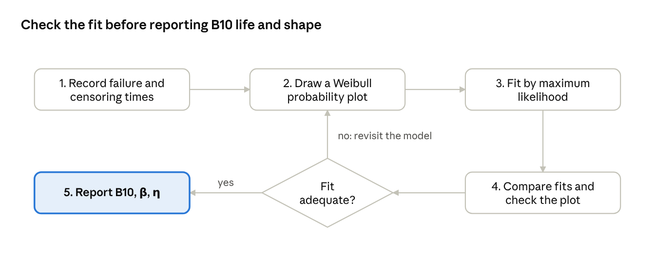
1. Record censoring carefully
For every unit, record the time and its status (failed or suspended). Also note the failure mode, because different mechanisms can follow different distributions.
2. Draw a probability plot first
A Weibull probability plot places ln(−ln(1 − F)) against ln(time), where F is the estimated fraction failed. Points close to a straight line support a Weibull model, and the slope reflects β. With censored data, estimate F with a method that accounts for suspensions, such as Kaplan–Meier [6], rather than ranking the failures alone [9].
3. Fit by maximum likelihood
Maximum likelihood estimation uses failures and suspensions together and gives confidence intervals, for example by the likelihood-ratio method [3][4]. With few failures the intervals will be wide, and the manuscript should say so plainly. IEC 61649 sets out recognised procedures for Weibull analysis [8].
4. Check the fit and compare alternatives
Compare the Weibull fit with alternatives such as the lognormal, using an information criterion such as AIC [7] together with the probability plots. A curved or S-shaped plot often signals more than one failure mode. Analyse those modes separately rather than forcing them into a single model.
Reading the reliability curve
The reliability curve shows the probability that a unit survives beyond a given time. In the simulated example below (β = 2.5, η = 1,000 h), the curve falls slowly at first and then steeply. That shape is the signature of wear-out when β is above 1.
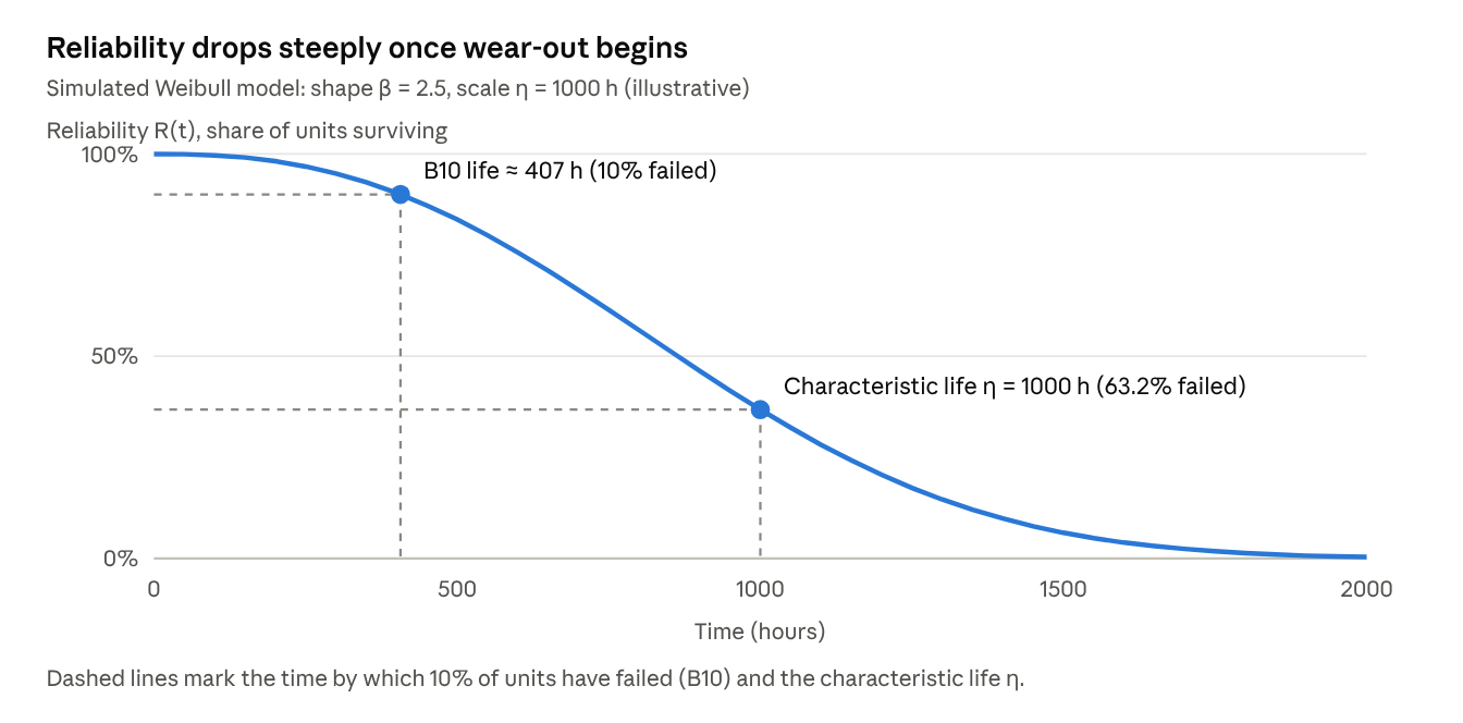
For design decisions, B10 life and its lower confidence bound usually matter more than average life. Avoid extrapolating far beyond the longest test duration, since the model cannot be checked there.
Reporting Weibull analysis in your manuscript
| Section | What to report |
|---|---|
| Methods | Test conditions, sample size, number of failures vs suspensions, failure definition, estimation method and software |
| Results | β and η with confidence intervals; B10 (and other percentiles) with intervals; the probability plot; a goodness-of-fit assessment |
| Discussion | Link β to the physical failure mechanism; state operating conditions and limits of validity |
| Supplementary data | List failure and suspension times so others can reproduce the analysis |
Common mistakes to avoid
- Discarding suspended units or treating them as failures
- Fitting a Weibull model without looking at the probability plot
- Mixing different failure modes in one fit
- Reporting point estimates without confidence intervals
- Extrapolating life far beyond the tested time
Frequently asked questions
What is censored data in reliability testing?
Units that had not failed when the test ended (or were removed for other reasons). Their survival time is known to be at least the stop time, and the analysis must use that information.
What does a Weibull shape parameter above 1 mean?
The failure rate rises with time, which points to wear-out mechanisms such as fatigue or corrosion.
What is B10 life?
The time by which 10% of units are expected to have failed. Report it with a lower confidence bound for design decisions.
Is least-squares regression on the probability plot acceptable?
It is still used, but maximum likelihood handles censored data better and gives confidence intervals directly, so most reviewers will expect it, especially with heavy censoring.
Related reading: Statistical reporting guidelines · Planning engineering PhD data collection in Saudi Arabia
Key takeaways
- Never drop units that were still running when the test stopped. They are censored data, not missing data.
- Look at a Weibull probability plot before fitting anything.
- Fit by maximum likelihood and report β, η and B10 life with confidence intervals.
- A curved plot usually means more than one failure mode. Separate them.
- Don’t extrapolate far beyond your longest test time.