Validating Physics-Informed Neural Networks for Reverse-Osmosis Membrane Fouling Prediction in Arabian Gulf Desalination Plants: Methodology for Sparse, High-Salinity Sensor Data

1. Why black-box fouling models get rejected

A purely data-driven model learns the operating envelope it was shown. Fouling is slow, drifting and partly unobserved, so the envelope moves — and the model has no internal reason to stay physically sensible when it does. Physics-informed neural networks add the governing equations to the training objective as a residual term, so the network is penalised for violating the physics as well as for missing the data [1].

That is the promise. The thesis must demonstrate that benefit through its validation design rather than assume it from the network architecture.

2. What goes in the loss: resistance-in-series, and the assumptions it hides

The physics residual should be derived from an explicitly stated transport relation. A resistance-in-series formulation expresses permeate flux as the effective driving force divided by the product of permeate viscosity and a sum of resistances:

R_m — the intrinsic hydraulic resistance of the clean membrane;
R_c — the resistance of a reversible cake or gel layer deposited on the surface, largely removed by cleaning;
R_f — the resistance of adsorptive or irreversible fouling, including pore-level deposition, not fully removed by cleaning.

Separating R_c from R_f is a modelling choice with consequences: it is what allows the model to represent incomplete recovery after a cleaning event, and a thesis that lumps them should say why.

For reverse osmosis, the driving force is not hydraulic pressure alone. The effective transmembrane driving force is the applied pressure difference minus the osmotic pressure difference across the membrane, which, at Gulf feed salinities, is a large term rather than a correction. Any concentration-polarisation or mass-transfer assumption — a film-model coefficient, a fixed polarisation factor, or none — should be stated explicitly rather than absorbed silently into the residual, because whatever is left unstated becomes something the network is free to learn around.

The approach is viable at both ends of the scale. A PINN built on Hermia’s four classical fouling equations, fitting a fractional weight for each mechanism, has identified which mechanism dominates flux decline and predicted decline from a much smaller dataset of over 50 flux-decline curves across more than ten studies [3]. At plant scale, a PINN embedding the solution-diffusion model of RO was trained on 760 days of records from a full-scale two-pass seawater plant, including two cleanings, reporting R² of 0.96 for permeate TDS and 0.97 for pressure drop [2].

3. Choosing the loss weight, and reporting it

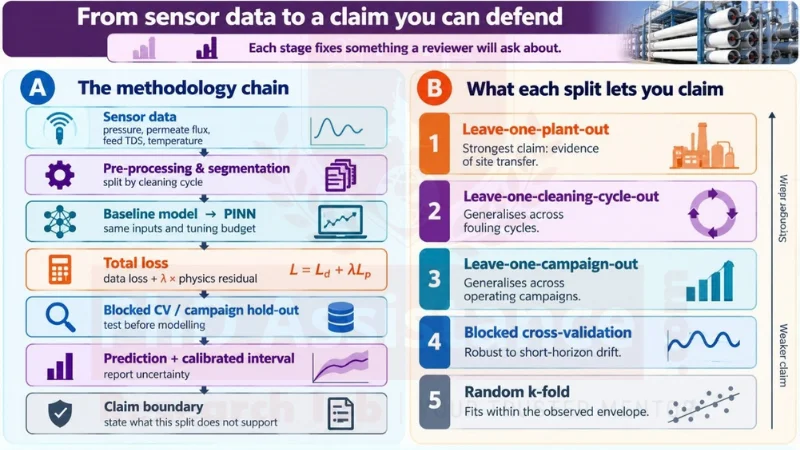
Figure 1. From sensor data to a claim you can defend. Panel A sets out the methodology chain, from cleaning-cycle segmentation through the two-term loss to an explicit claim boundary; Panel B shows the strongest claim each validation protocol supports. The figure is a design workflow and contains no plant data or results.

Total loss is the data mismatch plus a weighted physics residual. The loss weight is a consequential modelling decision that should be explicitly reported. In the plant-scale study above, the paper does not clearly specify how the two loss terms are weighted [2], which makes the physics contribution difficult to audit independently. A thesis should report the weight, the search used to choose it, and what happens to the solution when it is varied.

4. The baseline, and what counts as a benefit

A PINN should demonstrate a measurable benefit over a well-tuned conventional model under the same data, split and tuning budget. That benefit need not be limited to point-prediction accuracy; it may appear as better calibration, better physical consistency, better parameter identifiability, or greater robustness under distribution shift. A thesis that states in advance which of these it expects, and measures that, is stronger than one that reports RMSE alone.

The comparison is not a formality. A 2026 study comparing ridge-regularised multiple linear regression, an artificial neural network and support vector regression for transmembrane-pressure prediction at a seawater desalination plant found a best test R² of about 0.435 for SVR, with a wide bootstrap confidence interval and some cross-validation folds returning negative R² [7]. Conventional baselines on real plant data are neither trivially strong nor trivially weak, which is exactly why the comparison has to be run rather than assumed. The plant-scale SWRO PINN study, for its part, does not report a comparison against a purely data-driven baseline [2], so the proposition that physics improves generalisation is left open there.

5. Cleaning cycles are the unit of analysis

A cleaning event is a structural break, not a data point. The series before it, the event itself, the post-cleaning baseline and the subsequent trajectory are four distinct objects, and a model fitted across them without segmentation is fitting a discontinuity as if it were dynamics.

Four decisions belong in the written methodology: how each cleaning event is timestamped and verified against the plant log; what post-cleaning baseline becomes the new reference, and over what settling window; whether recovery is assumed complete, which the R_c/R_f split in §2 lets the model avoid assuming; and whether cycles are independent realisations or a sequence in which irreversible fouling accumulates. The last is a research question in its own right.

6. Splitting time-series data honestly

Random k-fold can place temporally adjacent and dependent observations in both training and validation folds, producing an optimistically biased estimate of generalisation when the process is drifting or serially dependent. Blocked cross-validation uses all the data while respecting temporal ordering, and has been recommended as the standard approach for time-series evaluation [5].

The potential effect of validation design on reported error has been demonstrated in cross-study membrane-fouling research. A 2026 analysis reported mean absolute errors of 0.08–0.14 in normalised-flux units under grouped cross-validation, where training and test samples come from the same experimental dataset, and stated that the MAE increased by approximately a factor of two when entire studies were excluded from training — concluding that differences between studies, rather than model capacity, limit predictive performance [4].

Validation protocol	What it tests	Main risk
Random k-fold	Interpolation within the observed envelope	Temporal leakage under drift
Blocked cross-validation	Robustness to short-horizon drift	May still reuse the same campaigns
Leave-one-campaign-out	Transfer across operating campaigns	Higher variance in the estimate
Leave-one-cleaning-cycle-out	Transfer across fouling cycles	Smaller effective sample
Leave-one-plant-out	Transfer across sites	Usually unavailable in practice

Prespecify the protocol before modelling, and report results under more than one so the reader can see the gap between them.

7. Identifiability: what the measurements can actually resolve

Accuracy is not identification. Before modelling, establish which quantities the instrumentation can resolve at all, and say so in the proposal:

Can fouling resistance be inferred uniquely, or only in combination with permeability decline?
Are viscosity and osmotic-pressure effects separable, given that both move with temperature and feed salinity?
Is the sampling frequency sufficient to resolve the dynamics the residual assumes?
Are multiple fouling mechanisms confounded within the available channels?
Can the model distinguish fouling from an operational change — a setpoint adjustment, a train being brought online, a feed-source switch?

Where a quantity is not identifiable, the options are to fix it from independent measurement, to reparameterise so only identifiable combinations are estimated, or to report a bounded rather than a point estimate. Discovering non-identifiability at the viva is the expensive route.

8. Sparse, high-salinity data: the Gulf-specific part

Salinity. Mean annual basin-wide salinity in the Gulf has been modelled at 40.5 g/kg [6], above open-ocean values, and the plant-scale SWRO record discussed above ran at a mean feed TDS of about 46,412 mg/L [2]. Higher feed salinity raises osmotic pressure, which enlarges the driving-force term in §2 and shifts the operating point, so coefficients fitted elsewhere should not be assumed to transfer.

The variables that carry Gulf conditions should be in the dataset explicitly rather than implied by location: feed temperature and its seasonal range; feed TDS and conductivity; turbidity or silt density index as an indicator of particulate load; applied feed pressure and transmembrane pressure; permeate flux, conductivity and recovery ratio; and pre-treatment state. Seasonal temperature swing matters because permeability is temperature-corrected, and a model trained on one season and tested on another is already attempting a transfer.

Sparsity. Plant instrumentation is built for control, not research: a handful of channels, coarse sampling, gaps during maintenance, and cleaning events logged inconsistently. This is where the physics term becomes a testable methodological hypothesis — embedding the residual may reduce the data requirement, which is what the small-dataset result in the mechanism-weighting study suggests [3], but it must be demonstrated on the thesis dataset rather than assumed.

9. Uncertainty quantification

For decision-oriented interpretation, point predictions should be accompanied by an explicitly defined uncertainty estimate, and the estimate should be checked rather than described. For a nominal 90% predictive interval, report empirical coverage on genuinely held-out observations and assess whether it is consistent with the intended nominal level. Because the data are temporally structured, state the calibration procedure and the dependence assumptions it relies on.

Distinguish aleatoric uncertainty, from sensor noise and process variability, which more data will not remove, from epistemic uncertainty, from limited coverage, which it may. The study should also test whether uncertainty increases appropriately as predictions move toward or outside the training distribution — behaviour to be demonstrated, not assumed.

10. Data access and instrumentation

This is the feasibility gate, settled before the proposal is written. A credible study needs multi-month operating records, a timestamped cleaning log and feed-water quality at a usable frequency. Access to Gulf plant operating data is a major feasibility risk for this design, and no established research-access route was identified in the sources reviewed for it. Work down this order: a collaboration agreement with an operator or utility, with a named contact and written terms; a pilot or university RO rig, accepting it is not a full-scale plant; and a study on published datasets, declared as such. Operating data is commercially sensitive — settle non-disclosure, reporting granularity and publication rights before collection.

11. What the result supports, and what it does not

A low physics residual means the network did not violate the equation that was supplied. If that equation omits a mechanism present in the plant, the residual is silent about it. Mapping results to claims explicitly is the cheapest defence available at examination.

Result obtained	Claim it supports	Claim it does not support
Lower error than the baseline	Better prediction under the tested split	Universal superiority of PINNs
Lower physics residual	Closer compliance with the specified equation	Physical correctness of the model
Good campaign hold-out performance	Generalisation across operating campaigns	Transfer to other plants or regions
Calibrated intervals on held-out data	Better-calibrated uncertainty under that scheme	Correct uncertainty everywhere
Consistent multi-plant validation	Evidence of site transfer	Universal applicability

The plant-scale study is explicit that its results are “firmly related to the specific RO desalination plant” where the data were collected [2] — a model of how to state a scope limit.

12. Study design checklist

Dimension	Evidence to hold before submission	Risk if unresolved
Residual form	The transport relation, resistances and osmotic term, written and justified	Physics term is decorative
Assumptions	Concentration-polarisation and mass-transfer treatment stated	Unstated physics learned around
Cleaning cycles	Segmentation rule and post-cleaning baseline defined	A discontinuity fitted as dynamics
Loss weight	Value, selection method, sensitivity run	Physics contribution unauditable
Baseline	A tuned conventional model on the same split [7]	The PINN’s benefit untested
Split	Results under at least two protocols [4,5]	Optimistic error read as generalisation
Identifiability	A stated answer for each model quantity	Parameters estimated that the data cannot resolve
Uncertainty	Interval method plus measured empirical coverage	Intervals that mean nothing
Data access	A named contact and a signed agreement	A major feasibility risk

13. Research questions

RQ1 (primary): does embedding a resistance-in-series residual provide a measurable benefit over a tuned conventional baseline on the same plant data and the same validation split, in accuracy, calibration or physical consistency? Comparison, not assumption. RQ2: how much does predictive error change between random k-fold, blocked time-series and leave-one-campaign-out validation? RQ3: how does the loss weight affect accuracy and the physical plausibility of the recovered fouling resistance? RQ4: are the model’s predictive intervals empirically calibrated on held-out operating periods? RQ5 (exploratory): is the split between reversible and irreversible fouling resistance identifiable from the available channels across successive cleaning cycles? RQ6 (exploratory): does the physics term reduce the quantity of labelled data needed to reach a stated accuracy [3]?

14. Contribution, and what a reviewer will ask

A completed thesis would deliver a PINN with its residual, assumptions, weight and split protocol fully specified; a fair comparison against a conventional baseline; error reported under multiple splits; calibrated uncertainty; and an explicit statement of identifiability. Coverage bounds generalisation, and no conclusion about any commercial membrane or plant is supportable from one site.

Common weaknesses that require revision: random k-fold on a drifting series; no baseline; an unreported loss weight; a residual that omits the osmotic term or the dominant fouling mechanism; cleaning events modelled as ordinary observations; uncalibrated intervals; and a single-plant result presented as a general method.

Need to validate your PINN research design before data collection?

PhD Assistance can review the proposed physics residual, the loss formulation, the validation split, the baseline comparison and the uncertainty treatment to identify methodological weaknesses while they are still cheap to fix.

Request a PINN Research Design Review with PhD Assistance’s research-methodology team. You receive a written recommendations summary for a supervisor meeting, covering whether the proposed model components are identifiable from the measurements you will actually have, whether the validation design supports the generalisation claim you intend to make, and what must be in place before modelling begins. The consultation advises on methodology; you carry out the research.

Frequently asked questions

Does a PINN need less data than a conventional model?

It may, and that is a question worth testing rather than a property to assume. A mechanism-weighting PINN reported accurate flux-decline prediction from a much smaller dataset [3], but the saving depends on how much of the behaviour the residual actually captures. Make it a research question rather than a premise.

Why is random k-fold cross-validation problematic for drifting fouling data?

Because it can place temporally adjacent and dependent observations in both training and validation folds, giving an optimistically biased estimate of generalisation. Blocked cross-validation respects the ordering while still using all the data [5], and campaign-level hold-out tests the thing a reviewer actually doubts.

Can a PINN trained on one desalination plant generalise to another plant?

Not automatically. A single-plant study can establish performance under the tested plant conditions and validation protocol, but it cannot by itself establish transferability. Cross-plant validation, or an explicitly designed domain-shift experiment, is needed to support that claim.

Is a low physics residual evidence that the model is physically correct?

No. It is evidence the model did not violate the equation supplied. If that equation omits a mechanism present in the plant — or absorbs concentration polarisation implicitly — the residual will not reveal it, which is why the assumptions in §2 belong in the written design.

Reference

Raissi M, Perdikaris P, Karniadakis GE. Physics-informed neural networks: a deep learning framework for solving forward and inverse problems involving nonlinear partial differential equations. J Comput Phys. 2019;378:686–707. doi:10.1016/j.jcp.2018.10.045
Helali S, Albalawi S, Bel Hadj Ali N. Harnessing physics-informed neural networks for performance monitoring in SWRO desalination. Water. 2025;17(3):297. doi:10.3390/w17030297
Saeedi Garakani S, Chew JW. Development of physics-informed machine-learning models to enhance understanding and prediction of membrane fouling. J Membr Sci. 2025;728:124133. doi:10.1016/j.memsci.2025.124133
Alves CL, Weschenfelder SE, Cechinel MAP, et al. Physics-informed machine learning for cross-study prediction of oil–water membrane fouling. Sci Rep. 2026;16:24415. doi:10.1038/s41598-026-54120-z
Bergmeir C, Benítez JM. On the use of cross-validation for time series predictor evaluation. Inf Sci. 2012;191:192–213. doi:10.1016/j.ins.2011.12.028
Ibrahim HD, Eltahir EAB. Impact of brine discharge from seawater desalination plants on Persian/Arabian Gulf salinity. J Environ Eng. 2019. doi:10.1061/(ASCE)EE.1943-7870.0001604
Kherraf S, Abahdou F-Z, Benbouzid M, et al. Prediction of reverse osmosis membrane fouling using machine learning: MLR, ANN, and SVM at a seawater desalination plant. Eng. 2026;7(3):106. doi:10.3390/eng7030106