Bayesian Calibration of Building Energy Models Against Smart-Meter Data: An Uncertainty-Aware UK PhD Methodology

Unsupervised Domain Adaptation

1. Why is the performance gap a research problem, not a slogan

The discrepancy between predicted and measured building energy performance is well documented, and a published framework distinguishes its components—the credibility gap in design, the gap between regulatory calculation and real operation, and the gap between simulation and measurement [1]. Treating these as one number is the first mistake.

The second mistake is assuming that the gap is universal. A study of 97 UK Passivhaus dwellings across 13 sites found no statistically significant difference between predicted and measured space-heating demand: 10.8 against 11.7 kWh/m²/yr, p = 0.43 [2]. The gap is a property of design, construction and modelling practice, not an inevitable feature of buildings — which makes explaining it a doctoral question rather than a lament.

Measurement itself carries quantified variability. In-use heat transfer coefficients across 19 occupied UK dwellings showed coefficients of variation of 1.0–11.8%, mean 7.1%, with boundary-condition models explaining around 85% of the observed variability [3]. An uncertainty-aware calibration must reflect this and distinguish measurement error from boundary-condition variability, rather than pooling both into observation noise.

2. What calibration currently means, and why fit is not enough

Deterministic calibration approaches often tune inputs until error metrics meet predefined thresholds of the kind set out in industry guidelines. A review of methods for matching simulation models to measured data identifies the weakness: such deterministic criteria can ignore input uncertainty and meeting them produces numerous models of the same building that can all be considered calibrated while representing different physical realities [4]. This is an equifinality problem, and further tuning does not resolve it.

Approach	What it produces	What it cannot tell you
Manual or expert tuning	One model meeting error thresholds	Which of many equally-fitting models is right; no input uncertainty
Automated optimisation	One best-fitting parameter set	Whether the optimum is unique; nothing about confidence
Bayesian calibration, no discrepancy term	Posterior distributions over parameters	Parameters absorb structural model error and are biased [6]
Bayesian calibration with discrepancy [5]	Joint posterior over parameters and discrepancy	Parameter recovery remains unresolved unless the discrepancy prior contains realistic identifying information (§5)

Calibration is not validation. Calibration asks whether parameter values are updated by the observed data; validation asks whether the resulting model predicts data not used for calibration. A model can fit calibration data well without demonstrating either parameter recovery or predictive validity, and the two questions need separate evidence.

3. Smart-meter data: what half-hourly readings can and cannot support

Half-hourly whole-premises consumption is rich in one dimension and poor in another. It resolves time well, letting a dynamic model be tested against driving conditions rather than annual totals. It does not disaggregate: one meter cannot separate fabric heat loss from occupant behaviour, appliance use or heating control, so a calibration assigning all residual variation to fabric parameters is an assumption, not a measurement. The choice of data streams materially affects what a calibration can recover [7].

Quantity	Whole-premises half-hourly meter	Additional evidence needed
Total electricity and gas use	Directly observed	—
Fabric heat loss	Indirect	Coheating or in-use HTC measurement [3]
Infiltration	Weakly identified	Airtightness testing
Occupancy and internal gains	Indirect	Survey or sensor data
Appliance loads	Indirect	End-use or sub-metered data
Heating control behaviour	Indirect	Controls or system monitoring

Three consequences. Match the model’s output resolution to the data’s. Treat occupancy and internal gains as uncertain quantities with priors, not fixed schedules. And decide in advance which periods calibrate and which are held out — heating and non-heating season data test different parts of the model.

4. The Bayesian calibration structure

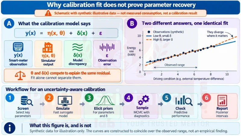
Research-design schematic titled “Why calibration fit does not prove parameter recovery”, labelled as a schematic with synthetic illustrative data that is not measured consumption and not a calibration result. Panel A sets out the calibration equation: a smart-meter observation equals simulator output at calibration parameters, plus a model discrepancy term, plus observation error, with each term glossed, and a highlighted note that the parameters and the discrepancy compete to explain the same residual so fit alone cannot separate them. Panel B plots synthetic observations with two fitted curves that coincide exactly over the observed range and diverge outside it, one implying low parameter values with small discrepancy and the other high parameter values with larger discrepancy, marked in the graphic as a synthetic example and not empirical results. A six-step workflow strip follows: screen, emulate, elicit priors, sample, check, report. A closing panel states that the synthetic curves were constructed to coincide, and that whether this confounding binds in any study is an empirical question.

Why calibration fit does not prove parameter recovery — a research-design schematic using synthetic illustrative data, not measured consumption and not a calibration result.

The framework that makes uncertainty explicit represents an observation as simulator output at calibration parameters, plus a discrepancy function capturing structural model error, plus observation error [5]. Each term takes a prior; the posterior is the joint distribution over parameters and discrepancy. This is the right structure — and adopting it is not the same as solving the problem.

5. The identifiability problem, stated plainly

Because the calibration parameters and the discrepancy function both explain residual variation, in the basic single-output calibration setup the data may not be sufficient to distinguish them without additional information. The consequence is established rather than speculative: ignoring model discrepancy yields biased and over-confident parameter estimates, while including it can improve predictive representation within the observed range but does not by itself establish recovery of the physical parameters unless realistic priors on the discrepancy are supplied [6]. The authors characterise this as a fundamental feature of inverse problems with mechanistic models.

The implication is sharp. A model calibrated to match the meter may extrapolate badly to the conditions a retrofit assessment cares about. As a research hypothesis rather than an established result, two calibrations with different fabric parameters and compensating discrepancy may fit identical data and imply different savings. Design to detect that, rather than assuming it away.

A worked illustration. Take three calibration parameters: wall U-value, infiltration rate and heating-system efficiency. Elicit a prior for each, run the calibration, and compare each posterior against its prior. If infiltration shifts substantially while wall U-value barely moves, the data informed infiltration more — and any conclusion resting on the U-value rests on the prior, not the meter. Repeat under a deliberately different discrepancy prior: if infiltration holds but efficiency moves with the discrepancy assumption, that tells the reader which conclusions are robust. Illustrative parameter names, not results.

Prespecify the identifiability checks. Report prior-versus-posterior comparisons for each parameter to show what the data actually updated; run synthetic-truth recovery experiments where the true parameters are known by construction; and report how posteriors move under alternative discrepancy priors. If a posterior barely moves from its prior, the data were uninformative about that parameter — and saying so is a result.

Identifiability is not fixed by priors alone. Additional measurement streams, multiple model outputs, constrained parameterisation and experimental design can each improve it [7]. A design that cannot identify a parameter from one meter should ask what evidence would.

6. Priors and identifiability: what the prior contributes

If the discrepancy prior is carrying part of the identification, it cannot be chosen casually.

Parameter priors should be elicited from building-physics evidence — measured U-values, airtightness results, published ranges for infiltration and system efficiency — with each source stated. A uniform prior over an implausibly wide range is not neutral: it claims extreme values are as likely as typical ones.

The discrepancy prior should encode what is believed about structural error: its smoothness, plausible magnitude, and whether it varies with external temperature or time of day. Document the reasoning and treat it as a sensitivity dimension, not a fixed input.

7. Making it computable: screening, emulation and the high-resolution likelihood

Screen first. Elementary-effects screening identifies which inputs materially affect the output at modest cost [8], reducing calibration to a small set of influential parameters. A parameter screened out is implicitly fixed, and that assumption should be stated.

Then emulate. A detailed dynamic simulation may be too computationally expensive to evaluate repeatedly during posterior sampling, so a Gaussian-process emulator trained on a designed sample of simulator runs replaces it. Published guidance for Bayesian calibration of building energy models covers these steps [9]. Report the emulator’s own validation on held-out runs, because emulator error propagates into the posterior.

High-resolution likelihood and temporal dependence. Half-hourly observations cannot automatically be treated as independent residuals: a single dwelling-year yields 17,520 observations per fuel, with daily, weekly and seasonal structure. The design should specify how temporal autocorrelation, missing readings, changing variance and that periodic structure are represented in the likelihood or residual model. Recent high-resolution work identifies exactly these obstacles — over-parameterisation and multiple solutions, surrogate models that do not capture temporal dynamics, and the computational burden of covariance calculations — and addresses them with sequence models and streamlined covariance computation [10]. If dimensionality reduction or representative temporal subsets are used for feasibility, prespecify the selection rule and report its effect on posterior inference.

8. Sampling, convergence and posterior predictive checking

Report the sampler, number of chains, length and burn-in, and formal convergence diagnostics rather than a visual impression of mixing [9]. Non-convergence is common with weakly identified parameters and is itself diagnostic information.

Then check the fitted model the way a Bayesian analysis should be checked: simulate from the posterior predictive distribution and compare against held-out periods not used in calibration. A model that reproduces its own training data proves little. A model that predicts held-out periods with appropriately calibrated uncertainty provides evidence of predictive performance beyond the calibration sample.

9. Evaluation: what the thesis must demonstrate

Report, at minimum: posteriors for all calibration parameters with their priors alongside; held-out posterior predictive performance, with interval coverage as well as central accuracy; the discrepancy posterior, so a reader sees how much work it is doing; and sensitivity of conclusions to the discrepancy prior.

Report the decision-relevant quantity with its uncertainty. If the purpose is retrofit assessment, the output is a predicted saving with a credible interval obtained by propagating the posterior — not a point estimate from one model. An interval spanning “worthwhile” and “not worthwhile” is an honest and useful result.

10. Data access, ethics and disclosure control

UK smart-meter data for research has a defined route rather than an improvised one. The SERL Observatory dataset provides half-hourly and daily electricity and gas data for over 13,000 households in Great Britain, linked to survey responses, Energy Performance Certificate records for a subset, and climate reanalysis variables [11]. Access runs through the UK Data Service secure environment under “five safes” controls.

Build the timeline into the research plan. Access requires Accredited Researcher status, university ethics approval, and project application review by the data service and the SERL Data Governance Board — together, researchers are advised to allow at least three months before data are needed. PhD students must have their supervisor as the project lead on the application, and outputs undergo statistical disclosure control before release [12].

Household energy data is personal data. Consumption traces reveal occupancy patterns. State what is reported at what granularity, and do not present dwelling-level results that could identify a household.

11. Bayesian calibration PhD study design checklist

Dimension	Evidence to hold before submission	Risk if unresolved
Data access	Accreditation, ethics approval and project approval, with the timeline costed	A major feasibility risk
Model and resolution	A named simulation tool, matched to the data’s time resolution	Calibration answers a question the data cannot
Parameter set	Screening results, with fixed parameters and their justification	Hidden assumptions presented as a calibration
Priors	Elicited parameter priors with sources, and a reasoned discrepancy prior	The prior silently carries the conclusion
Likelihood	A stated residual model for autocorrelation, missing data and changing variance	Standard errors and intervals understated
Emulator	Validation against held-out simulator runs	Emulator error misread as posterior uncertainty
Identifiability	Prior-versus-posterior comparison and synthetic-truth recovery	Fit reported as parameter recovery
Evaluation	Held-out posterior predictive checks with interval coverage	A model validated on its own training data

Any dimension without evidence behind it is a decision still to be taken or a limitation to declare — neither acceptable left unstated.

12. How to turn this blueprint into an approvable PhD proposal

Evidence gap map

Existing evidence	Main contribution	Remaining gap	How the proposed study addresses it
Performance-gap framework [1]	Decomposes the gap into distinct components	Conceptual; no estimation method	Supplies an estimation method for one named component
UK Passivhaus evidence [2]	Shows the gap is not universal	Specific construction standard; annual demand only	Tests at half-hourly resolution across a varied stock
In-use measurement variability [3]	Quantifies variability in measured HTC	Measurement-side; no model calibration	Separates measurement error from boundary-condition variability rather than treating both as observation noise
Calibration methods review [4]	Documents equifinality under deterministic criteria	Diagnoses; does not resolve identifiability	Treats identifiability as the object of study
Bayesian calibration framework [5]	The structure for parameters, discrepancy and error	Generic; not building- or stock-specific	Applies it with building-physics priors to UK dwellings
Model-discrepancy identifiability [6]	Shows parameter recovery requires realistic discrepancy priors	Statistical; no building application	Elicits and tests discrepancy priors for dwelling models
Data-stream influence [7]	Shows which data streams inform which parameters	Does not address stock-scale smart-meter constraints	Maps what one half-hourly meter can and cannot identify
High-resolution calibration [10]	Identifies temporal-dynamics and covariance obstacles	Method development; not UK dwelling stock	Applies a stated high-resolution likelihood to UK half-hourly data [11]

Research questions, with the inferential stance stated. RQ1 (primary): are the calibration parameters identified from half-hourly smart-meter data once a model discrepancy term is included — assessed by prior-versus-posterior movement and synthetic-truth recovery? This is an estimation and diagnosis question, not a hypothesis test. RQ2: how sensitive are the posteriors and the resulting predictions to the specification of the discrepancy prior and the residual model? RQ3: does the calibrated model predict held-out periods with well-calibrated uncertainty intervals? RQ4 (exploratory): how do posterior intervals on a decision-relevant quantity vary across dwelling types?

Contribution. A completed thesis would deliver a documented prior set for dwelling-model parameters and discrepancy; a reproducible screening, emulation and high-resolution likelihood pipeline; identifiability diagnostics reported as results rather than appendices; and posterior predictive performance on held-out data with interval coverage. Single-dataset coverage bounds generalisation, whole-premises metering bounds attribution, and no claim about an individual dwelling is supportable.

Common weaknesses that may require proposal revision: calibration criteria treated as validation; no discrepancy term, or one included without a reasoned prior; no screening, so dozens of parameters are calibrated against one meter; half-hourly residuals treated as independent; no emulator validation; no held-out evaluation; data access assumed; and a retrofit recommendation the design cannot support.

Frequently asked questions

Isn’t calibrating a model to measured data already standard practice?

Matching error thresholds is standard; showing the fitted parameters are identified is not. A review found such criteria admit many different models of the same building, all nominally calibrated [4]. The contribution is resolving that, not achieving the fit.

Why include a discrepancy term if it makes parameters harder to identify?

Omitting it does not remove structural error — it pushes it into the parameters, producing biased and over-confident estimates [6]. The term makes an existing problem visible and therefore addressable.

Can half-hourly data just be treated as independent observations?

No. A dwelling-year gives 17,520 readings per fuel with daily, weekly and seasonal structure, and recent high-resolution work identifies temporal dynamics and covariance computation as central obstacles [10]. The residual model is a design decision to be stated, not a default.

Can a thesis succeed if the parameters turn out not to be identified?

Yes, provided the diagnostics were prespecified. Establishing which parameters a half-hourly meter can and cannot inform, and what prior information or additional data streams [7] the rest would need, is a substantive methodological result.

Do I need stock-scale data, or will a few buildings do?

Both can be defensible, but they support different claims. A small, well-instrumented sample can support deeper identifiability analysis, whereas a larger dataset such as the SERL Observatory [11] can support analysis across dwelling types if its sampling and measurement limitations are appropriately addressed.

Can this work produce retrofit recommendations?

No. It produces calibrated models with quantified uncertainty and evidence on whether their parameters can be believed. Recommendations for any specific building require assessment by qualified professionals under the applicable standards.

Need a methodology review for your PhD calibration study?

If you are unsure whether your calibration design would survive an identifiability challenge — whether the priors are doing too much work, whether the residual model fits the data resolution, or whether the access route is realistic — that is what a methodology review is for.

What must be true before this PhD starts. A data access route with its timeline costed; university ethics approval planned ahead of application; a named simulation tool and model resolution; screening results; elicited priors with sources; a stated residual model; compute budget for emulation and sampling; and an identifiability-diagnostic plan. Each is a feasibility decision, not a formality.

Start a building-performance methodology consultation with PhD Assistance’s research-methodology team: a research-design review of your topic, data plan and calibration strategy against this framework, delivered as a written recommendations summary for a supervisor meeting. The consultation advises on methodology; you carry out the research.

Topic assessment — your question mapped against published performance-gap and calibration work, and where the novelty claim rests.
Data and model review — access route and timeline, simulation tool, resolution matching, residual structure and held-out design.
Statistical review — screening, emulation, prior elicitation, sampling diagnostics and identifiability checks.
Recommendations — what is defensible, what needs evidence and what to change.

To start, share your draft topic, target programme, and what you know about data access and ethics approval. The review supports your own work rather than replacing it, and provides no building or retrofit advice.

Reference

de Wilde P. The gap between predicted and measured energy performance of buildings: a framework for investigation. Autom Constr. 2014;41:40–49. doi:10.1016/j.autcon.2014.02.009
Mitchell R, Natarajan S. UK Passivhaus and the energy performance gap. Energy Build. 2020;224:110240. doi:10.1016/j.enbuild.2020.110240
Eastwood M, Allinson D, Li M, Roberts BM. Measuring the in-use thermal performance of dwellings: improving the precision by accounting for variability. J Build Phys. 2026;49(4):530–555. doi:10.1177/17442591251365953
Coakley D, Raftery P, Keane M. A review of methods to match building energy simulation models to measured data. Renew Sustain Energy Rev. 2014;37:123–141. doi:10.1016/j.rser.2014.05.007
Kennedy MC, O’Hagan A. Bayesian calibration of computer models. J R Stat Soc Series B Stat Methodol. 2001;63(3):425–464. doi:10.1111/1467-9868.00294
Brynjarsdóttir J, O’Hagan A. Learning about physical parameters: the importance of model discrepancy. Inverse Probl. 2014;30(11):114007. doi:10.1088/0266-5611/30/11/114007
Lim H, Zhai ZJ. Influences of energy data on Bayesian calibration of building energy model. Appl Energy. 2018;231:686–698. doi:10.1016/j.apenergy.2018.09.156
Morris MD. Factorial sampling plans for preliminary computational experiments. Technometrics. 1991;33(2):161–174.
Chong A, Menberg K. Guidelines for the Bayesian calibration of building energy models. Energy Build. 2018;174:527–547. doi:10.1016/j.enbuild.2018.06.028
Jiang G, Chen Y, Wang Z, Powell K, Billings B, Chen J. A deep learning-based Bayesian framework for high-resolution calibration of building energy models. Energy Build. 2024;323:114755. doi:10.1016/j.enbuild.2024.114755
Webborn E, Few J, McKenna E, Elam S, Pullinger M, Anderson B, Shipworth D, Oreszczyn T. The SERL Observatory dataset: longitudinal smart meter electricity and gas data, survey, EPC and climate data for over 13,000 households in Great Britain. Energies. 2021;14(21):6934. doi:10.3390/en14216934
Smart Energy Research Lab. Accessing SERL data — researcher accreditation, approval process and available datasets. Updated 22 September 2026. https://serl.ac.uk/researchers/