

Taxes and Entrepreneurship Research: Future Agenda for PhD Scholars
October 23, 2021
BLOCKCHAIN TECHNOLOGY USING ARTIFICIAL INTELLIGENCE FOR CARDIOVASCULAR MEDICINE
November 9, 2021How to Identify Right Performance Evaluation Metrics In Machine Learning Based Dissertation
Introduction
Every Machine Learning pipeline has performance measurements. They inform you if you’re progressing and give you a number. A metric is required for all machine learning models, whether linear regression or a SOTA method like BERT.
Every Machine Learning Activity, like performance measurements, can be split down into Regression or Classification. For both issues, there are hundreds of metrics to choose from, but we’ll go through the most common ones and the information they give regarding model performance. It’s critical to understand how your model interprets your data!
Loss functions are not the same as metrics. Loss functions display a model’s performance. They’re often differentiable in the model’s parameters and are used to train a machine learning model (using some form of optimization like Gradient Descent).Metrics are used to track and quantify a model’s performance (during training and testing), and they don’t have to be differentiable. If the performance measure is differentiable for some tasks, it may also be utilized as a loss function (possibly with additional regularizations), such as MSE.
PhD Assistance experts to develop new frameworks and novel techniques on improving the optimization for your engineering dissertation Services.
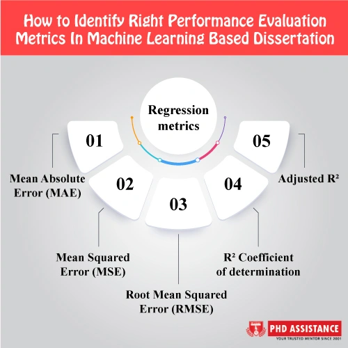
Regression metrics
The output of regression models is continuous. As a result, we’ll need a measure that is based on computing some type of distance between anticipated and actual values. We’ll go through these machine learning measures in depth in order to evaluate regression models:
- Mean Absolute Error (MAE)
The average of the difference between the ground truth and projected values is the Mean Absolute Error. There are a few essential factors for MAE to consider:
- Because it does not exaggerate mistakes, it is more resistant to outliers than MAE.
- It tells us how far the forecasts differed from the actual result. However, because MAE utilizes the absolute value of the residual, we won’t know which way the mistake is going, i.e. whether we’re under- or over-predicting the data.
- There is no need to second-guess error interpretation.
- In contrast to MSE, which is differentiable, MAE is non-differentiable.
- This measure, like MSE, is straightforward to apply.
Hire PhD Assistance experts to develop your algorithm and coding implementation on improving the secure access for your Engineering dissertation Services
- Mean Squared Error (MSE):
The mean squared error is arguably the most often used regression statistic. It simply calculates the average of the squared difference between the goal value and the regression model’s projected value. A few essential features of MSE:
- Because it is differentiable, it can be better optimized.
- It penalizes even minor mistakes by squaring them, resulting in an overestimation of the model’s badness.
- The squaring factor (scale) must be considered while interpreting errors.
- It’s indeed essentially more prone to outliers than other measures due to the squaring effect.
- Root Mean Squared Error (RMSE)
The square root of the average of the squared difference between the target value and the value predicted by the regression model is the Root Mean Squared Error. It corrects a few flaws in MSE.
A few essential points of RMSE:
- It maintains MSE’s differentiable feature.
- It square roots the penalization of minor mistakes performed by MSE.
- Because the scale is now the same as the random variable, error interpretation is simple.
- Because scale factors are effectively standardized, outliers are less likely to cause problems.
- Its application is similar to MSE.
PhD Assistance experts has experience in handling Dissertation And Assignment in cloud security and machine learning techniques with assured 2:1 distinction. Talk to Experts Now
- R² Coefficient of determination
The R2 coefficient of determination is a post measure, meaning it is determined after other metrics have been calculated. The purpose of computing this coefficient is to answer the question “How much (what percentage) of the entire variance in Y (target) is explained by variation in X (regression line)?”The sum of squared errors is used to compute this.
A few thoughts on the R2 results:
- If the regression line’s sum of Squared Error is minimal, R2 will be near to 1 (ideal), indicating that the regression was able to capture 100% of the variance in the target variable.
- In contrast, if the regression line’s sum of squared error is high, R2 will be close to 0, indicating that the regression failed to capture any variation in the target variable.
- The range of R2 appears to be (0,1), but it is really (-,1) since the ratio of squared errors of the regression line and mean might exceed 1 if the squared error of the regression line is sufficiently high (>squared error of the mean).
PhD Assistance has vast experience in developing dissertation research topics for students pursuing the UK dissertation in business management. Order Now.
- Adjusted R²
The R2 technique has various flaws, such as Deceiving The Researcher into assuming that the model is improving when the score rises while, in fact, no learning is taking place. This can occur when a model over fits the data; in such instance, the variance explained will be 100%, but no learning will have occurred. R2 is modified with the number of independent variables to correct this. Adjusted R2 is usually lower than R2 since it accounts for rising predictors and only indicates improvement when there is one.
Classification metrics
One of the most explored fields in the world is classification issues. Almost all production and industrial contexts have use cases. The list goes on and on: speech recognition, facial recognition, text categorization, and so on.
We need a measure that compares discrete classes in some way since classification algorithms provide discrete output. Classification Metrics assess a model’s performance and tell you if the classification is excellent or bad, but each one does it in a unique way.
So, in order to assess Classification models, we’ll go through the following measures in depth:
- Accuracy
The easiest measure to use and apply is classification accuracy, which is defined as the number of correct predictions divided by the total number of predictions, multiplied by 100.We may accomplish this manually looping between the ground truth and projected values, or we can use the scikit-learn module .
- Confusion Matrix (not a metric but fundamental to others)
The Ground-Truth Labels vs. Model Predictions Confusion Matrix is a tabular representation of the ground-truth labels vs. model predictions. The examples in a predicted class are represented by each row of the confusion matrix, whereas the occurrences in an actual class are represented by each column. The Confusion Matrix isn’t strictly a performance indicator, but it serves as a foundation for other metrics to assess the outcomes.We need to establish a value for the null hypothesis as an assumption in order to comprehend the confusion matrix.
- Precision and Recall
Type-I mistakes are the subject of the precision metric (FP). When we reject a valid null Hypothesis(H0), we make a Type-I mistake. For example, Type-I error mistakenly classifies cancer patients as non-cancerous. An accuracy score of 1 indicates that your model did not miss any true positives and can distinguish correctly between accurate and wrong cancer patient labeling. What it can’t detect is Type-II error, or false negatives, which occur when a non-cancerous patient is mistakenly diagnosed as malignant. A low accuracy score (0.5) indicates that your classifier has a significant amount of false positives, which might be due to an imbalanced class or poorly adjusted model hyper parameters.
The percentage of genuine positives to all positives in ground truth is known as the recall. The type-II mistake is the subject of the recall metric (FN). When we accept a false null hypothesis (H0), we make a type-II mistake. As a result, type-II mistake is mislabeling non-cancerous patients as malignant in this situation. Recalling to 1 indicates that your model did not miss any genuine positives and can distinguish properly from wrongly classifying cancer patients. What it can’t detect is type-I error, or false positives, which occur when a malignant patient is mistakenly diagnosed as non-cancerous. A low recall score (0.5) indicates that your classifier has a lot of false negatives, which might be caused by an unbalanced class or an untuned model hyper parameter. To avoid FP/FN in an unbalanced class issue, you must prepare your data ahead of time using over/under-sampling or focal loss.
- F1-score
Precision and recall are combined in the F1-score measure. In reality, the harmonic mean of the two is the F1 score. A high F1 score now denotes a high level of accuracy as well as recall. It has an excellent mix of precision and recall, and it performs well on tasks with unbalanced categorization.
A low F1 score means (nearly) nothing; it merely indicates performance at a certain level. We didn’t strive to perform well on a large portion of the test set because we had low recall. Low accuracy indicates that we didn’t get many of the cases we recognised as affirmative cases accurate.
However, a low F1 does not indicate which instances are involved. A high F1 indicates that we are likely to have good accuracy and memory for a significant chunk of the choice (which is informative). It’s unclear what the issue is with low F1 (poor accuracy or low precision). Is Formula One merely a gimmick? No, it’s frequently used and regarded a good metric for arriving at a choice, but only with a few changes. When you combine FPR (false positive rates) with F1, you can reduce type-I mistakes and figure out who’s to blame for your poor F1 score.
- AU-ROC (Area under Receiver operating characteristics curve)
AUC-ROC score/curves are also known as AUC-ROC score/curves. True positive rates (TPR) and false positive rates (FPR) are used .TPR/recall, on the surface, is the percentage of positive data points that are correctly classified as positive when compared to all positive data points. To put it another way, the higher the TPR, the fewer positive data items we’ll overlook. With regard to all negative data points, FPR/fallout refers to the fraction of Negative Data Points that are wrongly deemed positive. To put it another way, the greater the FPR, the more negative data points we’ll miss.
We first compute the two former measures using many different thresholds for the logistic regression, and then plot them on a single graph to merge the FPR and the TPR into a single metric. The ROC curve represents the result, and the measure we use is the area under the curve, which we refer to as AUROC.
A no-skill classifier is one that cannot distinguish between classes and will always predict a random or constant class. The proportion of positive to negative classes affects the no-skill line. It’s a horizontal line with the ratio of positive cases in the dataset as its value. It’s 0.5 for a well-balanced dataset. The area represents the likelihood that a randomly chosen positive example ranks higher than a randomly chosen negative example (i.e., has a higher probability of being positive than negative).As a result, a high ROC merely implies that the likelihood of a positive example being picked at random is truly positive. High ROC also indicates that your algorithm is good at rating test data, with the majority of negative instances on one end of a scale and the majority of positive cases on the other.
When your problem has a large class imbalance, ROC curves aren’t a smart choice. The explanation for this is not obvious, but it can be deduced from the formulae; you can learn more about it here. After processing an imbalance set or utilizing focus loss techniques, you can still utilise them in that circumstance. Other than academic study and comparing different classifiers, the AUROC measure is useless.
Conclusion
I hope you now see the value of performance measures in model evaluation and are aware of a few odd Small Techniques For Deciphering your model. One thing to keep in mind is that these metrics may be tweaked to fit your unique use case. Take, for instance, a weighted F1-score. It calculates each label’s metrics and determines their average weight based on support (the number of true instances for each label).A weighted accuracy, or Balanced Accuracy in technical words, is another example. To cope with unbalanced datasets, balanced accuracy in binary and multiclass classification problems is employed. It’s defined as the average recall in each category.
About Phdassistance
Ph.D. assistance expert helps you for research proposal in wide range of subjects. We have a specialized academicians who are professional and qualified in their particular specialization, like English, physics, chemistry, computer science, criminology, biological science, arts and literature, law ,sociology, biology, law, geography, social science, nursing, medicine, arts and literature, computer science, software programming, information technology, graphics, animation 3D drawing, CAD, construction etc. We also serve some other services as ; manuscript writing service, coursework writing service, dissertation writing service, manuscript writing and editing service, animation service.
REFERENCE
- Zhou, J., Gandomi, A. H., Chen, F., & Holzinger, A. (2021). Evaluating the quality of machine learning explanations: A survey on methods and metrics. Electronics, 10(5), 593.
- Huang, C., Li, S. X., Caraballo, C., Masoudi, F. A., Rumsfeld, J. S., Spertus, J. A., … & Krumholz, H. M. (2021). Performance Metrics for the Comparative Analysis of Clinical Risk Prediction Models Employing Machine Learning. Circulation: Cardiovascular Quality and Outcomes, CIRCOUTCOMES-120.
- Sanni, R. R., & Guruprasad, H. S. (2021). Analysis of Performance Metrics of Heart Failured Patients using Python and Machine Learning Algorithms. Global Transitions Proceedings.
- Anderson, David R., et al. Statistics for Business and Economics. Cengage Learning, 2020.