The advancement and challenges in computational physics

Introduction

For the last five decades, computational physics has been a valuable scientific instrument in physics. In comparison to using only theoretical and experimental approaches, it has enabled physicists to understand complex problems better. Computational physics was mostly a scientific activity at the time, with relatively few organised undergraduate study. Students were supposed to pick up the requisite computational skills when they went through with their studies. This culminated in a small number of highly qualified computational physics graduates. This pattern has shifted dramatically in recent years, with increasingly sophisticated commercial applications or freeware computer programmes created by more specialised groups being used by computational physics research groups. The benefit is that a larger number of researchers now have access to more effective codes that integrate more sophisticated modelling of physical structures of interest [1]. This post discusses the advancement and challenges in computational physics.

A) Recent researches in computational physics

1.Python framework for computational physics

For rapid prototyping of the latest physics codes, a newly designed computational system was created. TurboPy is a lightweight physics simulation application that is built on the architecture of the particle-in-cell code turboWAVE. It implements a Simulation class that drives the simulation and maintains coordination between PhysicsModule class that handles the specifics of the dynamics of the different sections of the problem and a few other classes, including a Grid class and a Diagnostic class to handle various ancillary issues that occur frequently. Figure 1 depicts one possible implementation of this workflow as turboPy physics units. The workflow is split into two custom turboPy physics modules in this implementation [2].

Figure 1. Custom turboPy physics modules and diagnostics are included in this diagram to show one alternative implementation of the example workflow. Each box in the flow denotes a PhysicsModule or Diagnostic subclass that has been written to conduct the action mentioned. [2].

2.Machine Learning in Computational Physics

A new method for sampling training data based on a Taylor approximation is built to approximate physical simulation codes in machine learning. Though not specifically related to Deep Learning, an approach is used to approximate the solution of a physical ODE structure using a Deep Neural Network and improve its precision with the same model architecture. In addition to the reasons stated leads, the concept of using numerical simulation derivatives to improve ML model training should be investigated. Include derivatives as new teaching points to have a DNN learn these derivatives as an example of implementation. Figure 2 depicts a Taylor sampling algorithm [3].

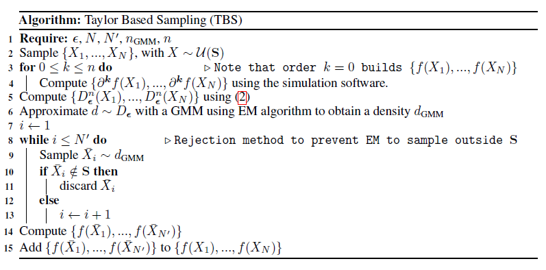
Figure 2. A Taylor based sampling algorithm [3]

3.Physics-informed neural networks for the incompressible Navier-Stokes equations

To overcome the limitations of simulating incompressible laminar and turbulent flows, physics-informed neural networks (PINNs) are used, which encode the governing equations directly into the deep neural network through automatic differentiation. The Navier-Stokes flow nets (NSFnets) were created using two different mathematical formulations of the Navier-Stokes equations: the velocity-pressure (VP) and the vorticity-velocity (VV) formulations. Even though this is a new methodology, a standard benchmark problem is used to assess the precision, convergence rate, computational cost, and flexibility of NSFnets; analytical solutions and direct numerical simulation (DNS) databases provide suitable initial and boundary conditions for NSFnet simulations. The ability to use NSFnets for applications other than classical CFD was shown in this study, such as solving ill-posed (noisy or incomplete boundary conditions) or inverse problems (unknown fluid properties) that would be impossible or prohibitively costly to solve using traditional approaches. We also use a basic example of transfer learning to demonstrate how we can reduce NSFnets’ comparatively high computational cost. The velocity-pressure (VP) form and the vorticity-velocity (VV) form of the unsteady incompressible three-dimensional Navier-Stokes equations, as well as their corresponding physics-informed neural networks (PINNs), were introduced in this work (Figure 3) [4].

Fig. 3. A schematic of NSFnets [4]

B) Computational physics & its challenges

Despite the “early adopters” of computational physics described above and individuals’ desire to transform computer science into physics analysis, society requires a (new) space to share ideas and insight. Any efforts, such as the Program Library of Computer Physics Communications, have been popular today. However, such collections must expand in-depth, provide more groups, and go beyond just storing code libraries. Furthermore, the distance between available and validated statistical methodologies and their application in computational physics inevitably expands: computer scientists and applied mathematicians have never been more efficient than they are now. How will the (computational) physics world as a whole deal with the rapid development in fields that serve as a methodological foundation? In physics, the mathematical representation of NP has long been the basic language. Computation enables the solution of ever more complicated mathematical models, reinforcing the mathematical language’s strength. This shows how the synergy effect enhances a specific region. However, taking advantage of such an advantage poses a significant risk in and of itself. The Intergovernmental Panel on Climate Change’s (IPCC) global weather simulations is an example of a move above scientists in either theory or experiments joined by computation and trying to interact [5].

 Conclusion

The enormous progress made in applied mathematics, numerics, and computer science is compared with the progress made in computational physics. Although physicists are mostly concerned with their original experiments on physical problems, they cannot keep up with the latest developments of numerical analysis on their own. Consequently, we see a growing difference between theoretical findings on the one side and the application and use of analytical methods focused on those concepts on the other. Closing this gap, i.e., introducing modern methods faster and more consistently and integrating them into successful computational physics science, seems to be one of the major challenges. A (computational) physicist’s ability to recognise emerging concepts in applied mathematics, numeric, and computer science and then convert them into research projects is particularly difficult. To identify the potential of a new analytical instrument, a computational physicist will need to be interested in two different scientific groups, create benchmarks and other parameters to judge the applicability of a method, and then apply and test the findings using his or her knowledge in a subfield of physics.

Reference

[1] T Salagaram and N Chetty 2013 J. Phys.: Conf. Ser. 454 012075.

[2] A.S. Richardson, D.F. Gordon, S.B. Swanekamp, I.M. Rittersdorf, P.E. Adamson, O.S. Grannis, G.T. Morgan, A. Ostenfeld, K.L. Phlips, C.G. Sun, G. Tang, D.J. Watkins, TurboPy: A lightweight python framework for computational physics, Computer Physics Communications, Volume 258, 2021, 107607, https://doi.org/10.1016/j.cpc.2020.107607.

[3] Paul Novello, Gaël Poëtte, David Lugato, Pietro Congedo. A Taylor Based Sampling Scheme for Machine Learning in Computational Physics. 2019. arXiv:2101.11105

[4] Xiaowei Jin, Shengze Cai, Hui Li, George Em Karniadakis, NSFnets (Navier-Stokes flow nets): Physics-informed neural networks for the incompressible Navier-Stokes equations, Journal of Computational Physics, Volume 426, 2021, 109951, https://doi.org/10.1016/j.jcp.2020.109951.

[5] Klingenberg C (2013) Grand challenges in computational physics. Front. Physics 1:2. doi: 10.3389/fphy.2013.00002